From Transformer to ChatGPT
going back in time in order to move forward
Attention is all you need
Since their introduction in 2017, transformers
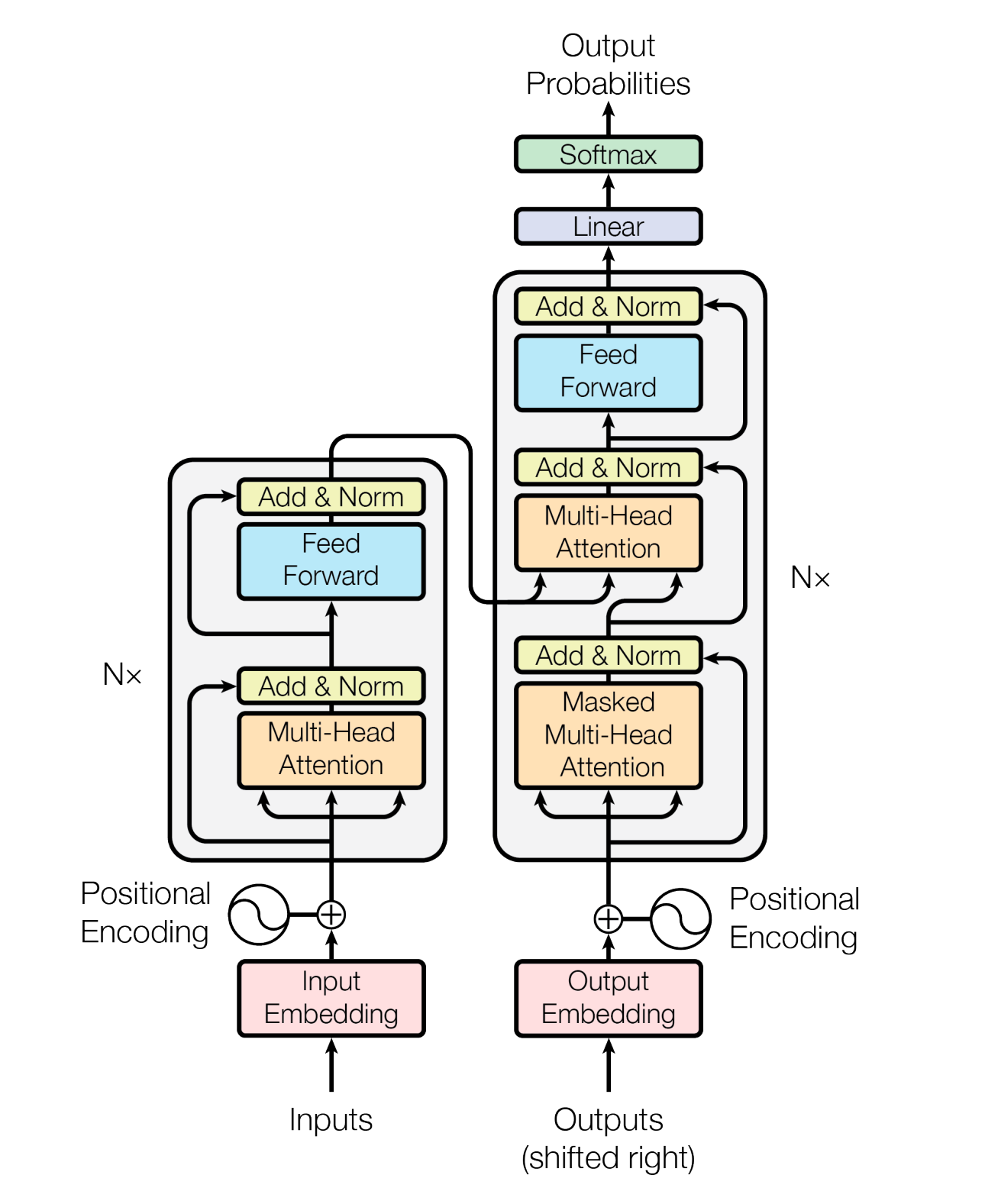
On a high level, transformers represents an efficient, optimizable, general-purpose neural network. They are designed to encode and decode sequences of data, allowing individual tokens to interact and communicate with one another.
Attention mechanism
The attention mechanism lets us model dependencies between words regardless of their position in the sequence. It was first introduced by Bahdanau et al.
a fixed-length vector is a bottleneck in improving the performance of this
basic encoder–decoder architecture, and propose to extend this by allowing
a model to automatically soft-search for parts of a source sentence that
are relevant to predicting a target word, without having to form these
parts as a hard segment explicitly.
The attention mechanism compares intermediate representations $h_i$ developed in the decoder with encoded inputs $z_j$ and outputs $z_j$ that is closest to $h_i$. Basic attention mechanism in transformers:
\[\begin{aligned} o_i & =\sum_{j=1}^n \alpha_{i j} z_j \\ \alpha_{i j} & =\frac{\exp \left(z_j^{\top} h_i / \sqrt{d_k}\right)}{\sum_{j^{\prime}=1}^n \exp \left(z_{j^{\prime}}^{\top} h_i / \sqrt{d_k}\right)} \end{aligned}\]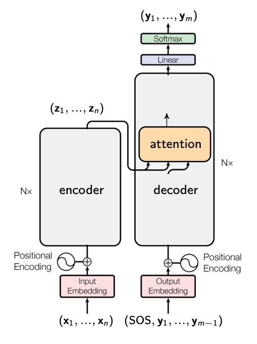
$d_k$ is the dimensionality of the $z_j$ and $h_i$.
This is called scaled-dot attention.
We can think of the scaled dot-product attention as finding values $v_j=z_j$ with keys $k_j=z_j$ that are closest to query $q_i=h_i$. Re-writing the scaled dot-product attention using keys, values and query:
\[\begin{aligned} o_i & =\sum_{j=1}^n \alpha_{i j} v_j \\ \alpha_{i j} & =\frac{\exp \left(k_j^{\top} q_i / \sqrt{d_k}\right)}{\sum_{j^{\prime}=1}^n \exp \left(k_{j^{\prime}}^{\top} q_i / \sqrt{d_k}\right)} \end{aligned}\]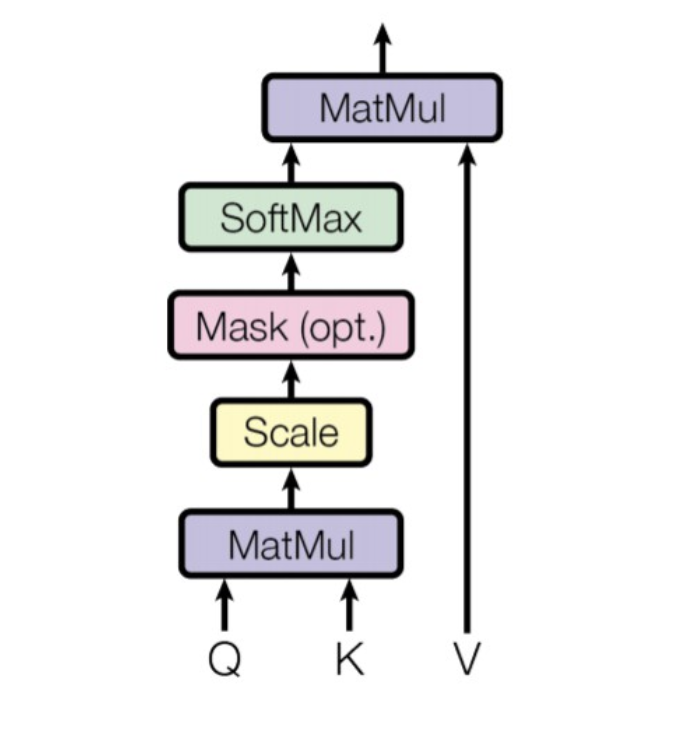
in the matrix form:
\[\begin{gathered} \\ \qquad \operatorname{attention}(Q, K, V)=\operatorname{softmax}\left(\frac{Q K^{\top}}{\sqrt{d_k}}\right)\\ \\ V \in R^{m \times d_v}, Q \in R^{n \times d_k}, K \in R^{m \times d_k} \end{gathered}\]Multihead attention
Instead of doing a single scaled dot-product attention, it is more beneficial to project keys, queries and values into lower-dimensional spaces, perform scaled dot-product attention there and concatenate the outputs
\[\begin{gathered} \operatorname{head}_i=\operatorname{attention}\left(Q W_i^Q, K W_i^K, V W_i^V\right) \\ \\ \operatorname{MultiHead}(Q, K, V)=\text { Concat }\left(\operatorname{head}_1, \ldots, \text { head }_h\right) W^O \\ \\ V \in R^{m \times d_v}, Q \in R^{n \times d_k}, K \in R^{m \times d_k} \\ \\ \text { head }_i \in R^{n \times d_i}, \text { output } \in R^{n \times d_k} . \end{gathered}\]
Self-Attention
Attention is all you need: Use the same multi-head attention mechanism to convert inputs $(x_1, \ldots, x_n)$ into representations $(z_1, \ldots, z_n)$.
For simplicity, assume that we use scaled dot-product attention:
\[z_i=\sum_{j=1}^n \alpha_{i j} x_j \quad \alpha_{i j}=\frac{\exp \left(x_j^{\top} x_i / \sqrt{d_k}\right)}{\sum_{j^{\prime}=1}^n \exp \left(x_{j^{\prime}}^{\top} x_i / \sqrt{d_k}\right)}\]
Here, we use vectors $x_i$ as keys, values and queries. This is called self-attention.
Advantage over RNN: The first position affects the representation in the last position (and vice versa) already after one layer! (think how many layers are needed for that in RNN or convolutional encoders).
Transformer encoder
After self-attention, the representation in each position is processed with a mini-MLP (Feed Forward block in the figure). The encoder is a stack of multiple such blocks (each block contains an attention module and a mini-MLP).

Transformer decoder
When predicting word $y_i$ we can use the preceding words $y_1$, …, $y_{i-1}$ but not subsequent words $y_i$, …, $y_m$. Again, attention-is-all-you-need idea: Use self-attention as a building block of the decoder. We need to make sure that we do not use subsequent inputs $y_i$, …, $y_m$ when producing output $o_i$ at position $i$. This is done using masked self-attention

For simplicity, assume that we use scaled dot-product attention:
\[h_i=\sum_{j=1}^m \alpha_{i j} v_j \quad \alpha_{i j}=\frac{\exp \left(v_j^{\top} v_i / \sqrt{d_k}+m_{i j}\right)}{\sum_{j^{\prime}=1}^m \exp \left(v_{j^{\prime}}^{\top} v_i / \sqrt{d_k}+m_{i j^{\prime}}\right)}\]We want not to use subsequent positions
\(v_{i+1}, \ldots, v_m\) when computing output $h_i$. We can do that using attention masks $m_{i j}$:
\[\begin{aligned} & m_{i j}=0, \text { if } j \leq i \\ & m_{i j}=-\infty \text { and therefore } \alpha_{i j}=0, \text { if } j>i \end{aligned}\]After self-attention (where a model assesses relationships and dependencies within a single sequence of data) and cross-attention (where a model assesses relationships and dependencies across different sequences or sources), the representation in each position is processed with a mini-MLP (Feed Forward block in the figure). The decoder is a stack of multiple such blocks (each block contains two attention modules and a mini-MLP).

Positional encoding
Since transformers don’t use previous data or patterns to understand the order of things, we have to add extra information to show where each part of the sequence stands in relation to the others. Vaswani et al., 2017 used hard-coded (not learned) positional encoding.:
\[\begin{aligned} & PE(p, 2 i) =\sin \left(p / 10000^{2 i / d}\right) \\ & PE(p, 2 i+1) =\cos \left(p / 10000^{2 i / d}\right) \end{aligned}\]where $p$ is position, $i$ is the element of the encoding. This encoding has the same dimensionality $d$ as input/output embeddings. This encoding has the same dimensionality d as input/output embeddings.
End note
Encoder-decoder architecture
Transformer layers with Multi-Head Self-Attention and Feed-Forward sublayers
Transformer Decoder layers also have Encoder-Decoder Attention sublayer
N Encoder and Decoder layers (N=6 in the paper)
Attention uses queries and key-value pairs to produce weighted sums of the values
Feed-Forward layers then process the inputs independently for better representations
Trained end-to-end for translating sequences
Superior performance over RNNs
If you have trouble understanding the model still, consider looking at this Annotated Transformer blog post.
Improving Language Understanding by Generative Pre-Training (GPT-1)
OpenAI introduced the first version of GPT (Generative Pre-Trained Transformer)
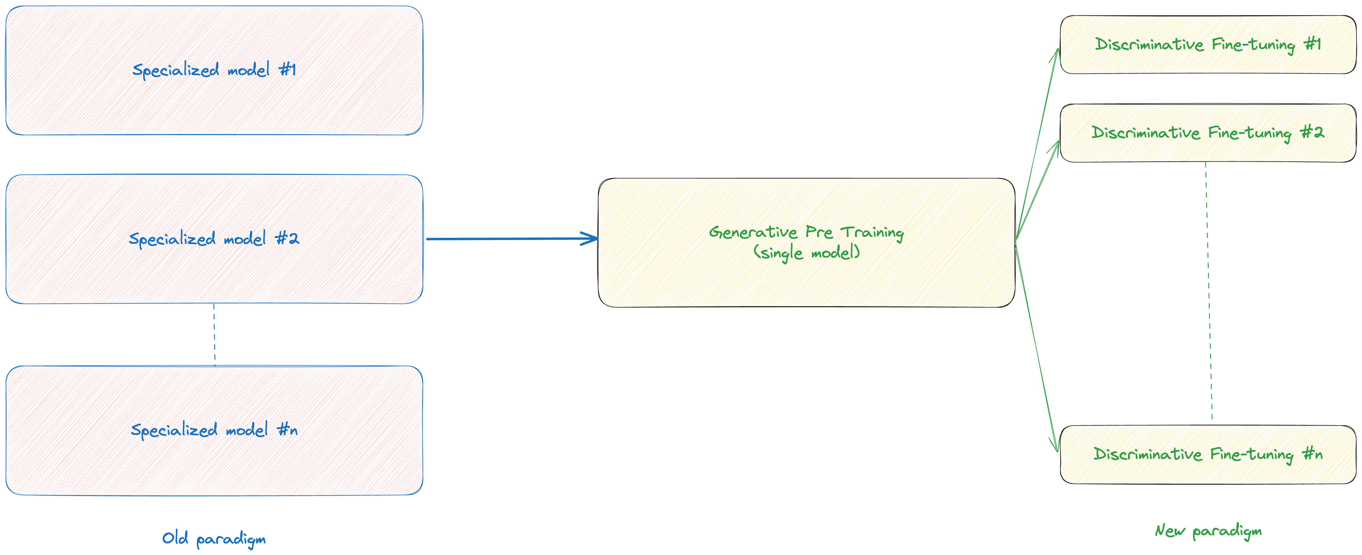
Introducing a new paradigm
Most deep learning methods require substantial amounts of manually labeled data, which restricts their applicability in many domains that suffer from a dearth of annotated resources.
Which raises the following questions:
- Is it feasible to extract learning from raw text without relying on translated sentence pairs?
- What are the most effective objectives to employ in this context?
- What strategies should we adopt to effectively transfer acquired knowledge to the specific tasks that matter to us?
- To what extent does modeling language contribute practically to solving various NLP tasks?
Tokenization
Imagine our corpus has the following words
"from", "transformer", "to", "chatgpt"
then our base vocabulary will be
['a', 'c', 'e', 'f', 'g', 'h', 'm', 'n', 'o', 'p', 'r', 's', 't']
For real-world use cases, base vocabulary will contain all the ASCII characters, and maybe some Unicode characters as well. If an example you want to tokenize uses a character that is not in the training corpus, that character will be converted to unknown tokens. That’s one reason why lots of NLP models are bad at analyzing content with emojis, e.g.
Good characteristics of good vocabulary
- Be able to represent all characters and symbols that exist in digital format
- The vocabulary should be as expressive as possible (e.g. words are more expressive than characters)
Options
- Bytes: 2^8=256 possible tokens only, can represent anything, but not expressive
- Unicode codes (character level tokens): 130k+ tokens, too large!
- Words: more than 1M only in English vocabularies, too large and not flexible enough!
- Sub-words: fuzzy term to indicate anything from byte-pairs up to full words; can be crafted to satisfy all the desiderata above!
GPT paper used a technique called bytepair encoding (BPE) vocabulary with 40,000 merges. It’s a greedy data-compression technique that iterative replaces the most frequent pair of tokens in a sequence with a single unused token.
Procedure
- Initialize vocabulary V = {all possible bytes}
- Count the frequency of all unique subsequent pairs of tokens
- Substitute the most frequent pair with a new token and add the token to V (“merge” op.)
- Repeat 2. and 3. until the V size is reached or after N merges ops
How to implement BPE (character-level) in Python
Generative Pre-Training
Given an unsupervised corpus of tokens $U=\left{u_1, \ldots, u_n\right}$, they use a standard language modeling objective to maximize the following likelihood:
\[L_1(U)=\sum_i \log P\left(u_i \mid u_{i-k}, \ldots, u_{i-1} ; \Theta\right)\]where $k$ is the size of the context window, and the conditional probability $P$ is modeled using a neural network with parameters $\Theta$.
They use Decoder-only Transformer, a variant of Transformer as the base architecture, as its excellent for handling complex dependencies within sequences
\[\begin{aligned} h_0 & =U W_e+W_p \\ h_l & =\text { transformer_block }\left(h_{l-1}\right) \forall i \in[1, n] \\ P(u) & =\operatorname{softmax}\left(h_n W_e^T\right) \\ \\ \end{aligned}\]where $U=\left(u_{-k}, \ldots, u_{-1}\right)$ is the context vector of tokens, $n$ is the number of layers, $W_e$ is the token embedding matrix, and $W_p$ is the position embedding matrix.

Discriminative fine-tuning

After pre-training the model, the parameters are adapted to supervised target task. Assume label set $C$, a sequence of input tokens $x^1, \ldots, x^m$, along with a label $y$. The inputs are first converted into an ordered sequence that our pre-trained model can process, passed through GPT to obtain the hidden representation of the last layer for the last token as the sequence representation, which is then fed into an added linear output layer with parameters W_y to predict y.
That gives the following language modelling objective to maximize:
\[L_2(\mathcal{C})=\sum_{(x, y)} \log P\left(y \mid x^1, \ldots, x^m\right) .\]They found that including language modeling as an auxiliary objective to the fine-tuning helped learning by (a) improving generalization of the supervised model, and (b) accelerating convergence. They optimize the following objective (with weight $\lambda$ ):
\[L_3(\mathcal{C})=L_2(\mathcal{C})+\lambda * L_1(\mathcal{C})\]The ony extra parameters required during fine-tuning are W_y, and embeddings for delimiter tokens.
The long-term vision
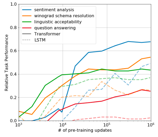
In order to understand why the pre-training of transformers is so effective, the authors used a series of heuristic solutions that use the underlying generative model only without supervised fine-tuning. The results show the performance is stable and increases over training suggesting that pre-training supports the learning of a wide variety of task relevant functionality. The vision is if we improve the performance of the model in the pre-training phase, it might become good enough to not require any fine-tuning!
Language Models are Unsupervised Multitask Learners (GPT-2)
Hypothesis: Language acts as a versatile medium that encodes tasks, inputs, and outputs into a uniform sequence of symbols.
For instance, a translation task can be represented as (translate to French, English text, French text), and similarly, a reading comprehension task as (answer the question, document, question, answer).
Given that the supervised learning objective simply narrows down the focus to a particular segment of this sequence, the ultimate goal—achieving the lowest error rate, known as the global minimum—remains the same for both supervised and unsupervised learning objectives. Consequently, a model trained on an unsupervised next-token prediction task inherently strives towards a goal that aligns with that of supervised tasks, suggesting that the model’s pre-training on diverse web data equips it with zero-shot transfer capabilities through an underlying meta-learning process during its generative pre-training.
With more than 10X the parameters and trained on more than 10X the amount of data, GPT-2 zero-shots to state of the art performance on 7 out of 8 tested language modeling datasets.
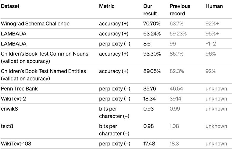

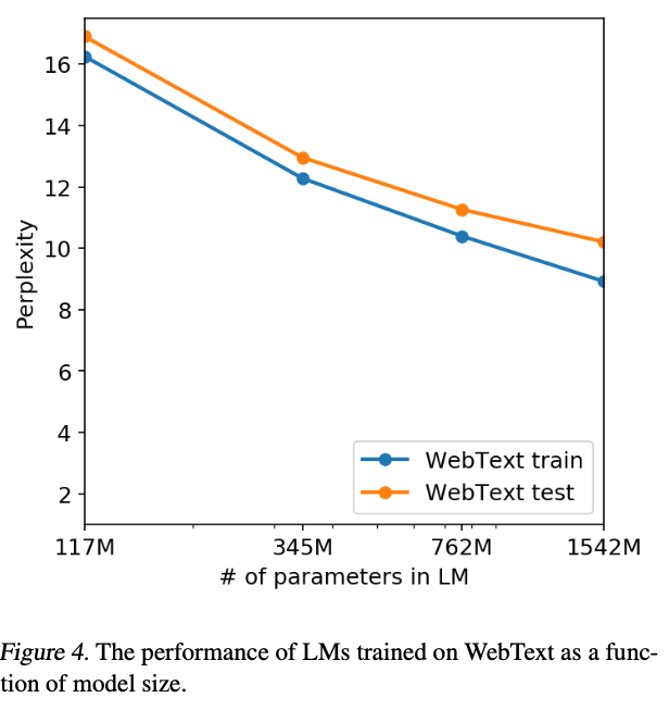
Looking at the above plot, we can clearly see more data + bigger models leads to better zero-shot abilities. And all models still underfit WebText, i.e. if trained for longer would get better test perplexity!
Note on perplexity
In Natural Language Processing (NLP), perplexity is a measurement of how well a probability model predicts a sample. It is commonly used to evaluate language models. Perplexity is defined as the exponentiation of the entropy of the probability distribution for a given test dataset.
Here’s a step-by-step breakdown of the calculation of perplexity for a language model:
-
Probability of the Sequence: First, compute the probability of the sequence of words (or tokens) according to the language model. This is often done by multiplying the probabilities of each word given the previous words in the sequence.
-
Calculate Entropy: The entropy of the sequence is the average negative log-probability of the test set sequences. For a sequence of words $W=w_1, w_2, \ldots, w_N$, the entropy $H$ is calculated as: \(H(W)=-\frac{1}{N} \sum_{i=1}^N \log _2 p\left(w_i \mid w_1, w_2, \ldots, w_{i-1}\right)\) where \(p\left(w_i \mid w_1, w_2, \ldots, w_{i-1}\right)\) is the probability of word $ w_i $ given the preceding words in the sequence.
-
Exponentiate the Entropy: Perplexity $P P$ is defined as the exponentiation of the entropy: \(P P(W)=2^{H(W)}\)
The intuition behind perplexity is that it measures how “perplexed” the model is when predicting new data; a lower perplexity indicates that the model is more confident in its predictions. In other words, a good language model will have a low perplexity, meaning that the sequences it predicts are relatively likely.
In this form, you don’t exponentiate the log probabilities but rather average them directly and then apply the exponentiation. This is mathematically equivalent to the original formula but is more practical for computational purposes.
Scaling Laws for Neural Language Models
The insights from the GPT-2 paper highlight the promising outcomes achieved through pre-training by increasing data volume and scaling the model size. This leads to key inquiries:
- What are the boundaries of improving performance through the combined effect of data and model scaling? To what extent can we push this?
- What are the resource implications, in terms of GPU hours and financial budget, for attaining specific performance levels? Within a defined budget, what is the optimal performance we can achieve?
Transformer LMs complexity
The number of parameters in a decoder-only transformer language is:
\[\text { Parameters }=12 n_{\text {layer }} d_{\text {model }}^2\]Roughly speaking, all parameters participate in 1 add and 1 multiply in a forward pass, and 2x in the backward pass, for every token. So training compute is:
\[\text { Compute }=6 P D\]where $P$ is the number of parameters in the model, and $D$ is the number of tokens you process.

Transformer LMs and Orders of Magnitude
The largest models we have so far has roughly in the order of 1 trillion ($1e^{12}$) parameters.
A100 GPUs performs ~ $3^{14}$ FLOPs or $2e^{19}$ FLOP/day, a PF-day is around ~ 3 A100 day $~8.6e^{19}$ FLOPs.
Largest Train Compute = $6 P D = 6^* 1 e^{12} * 3 e^{11}$ (same number of tokens GPT-3 was trained on)
Scaling laws
There are precise scaling laws for performance of ML models as functions of model size, dataset size, and the amount of compute used for training, with some trends spanning more than seven orders of magnitude. Other architectural details such as network width or depth have minimal effects within a wide range
To get scaling results, we can train many models of different sizes on different sized datasets. The performance of language models gets better consistently when you increase the size of the model, the dataset, and the computing power used in training. To get the best results, you need to increase all three together. When one of these factors isn’t limited by the others, its improvement follows a power-law trend.

You want to spend most of your compute on making the model bigger, around 2/3 on the geometric scale

Architecture you want to train on is less important, unless the architecture itself creates a bottleneck. You can of course still do language modelling with LSTMs instead of transformer. And you can see what you actually get using LSTMs instead of transformers.

At zeroth order, LSTMs did not seem too bad, and as you make them bigger, they are scaling up quite nicely. But there is a constant offset where transformers are five to ten times more efficient. Moreover, if we take a look at 1000 tokens, we can look at the losses as a function of the position in context. And we can see that LSTMs plateau quite quickly at around 100 tokens.
Language Models are Few-Shot Learners (GPT-3)
As discussed before, while using task-specific datasets and task-specific fine-tuning can bring strong performance on a desired task, its not the right way forward. Every new task requires a large dataset of labeled examples, which then will limit the applicability of language models. Now, using empirical scaling laws, we want to see how far we can get with task-agnostic architecture with larger model and more data.

As the results show, we can see that zero-shot performance is still not competitive with fine-tuned models. But by just providing examples of desired input-output behaviour in the prompt to the model, performance increases greatly without doing gradient updates.
Introducing the concept of in-context learning: using the text input of a pretrained language model as a form of task specification: the model is conditioned on a natural language instruction and/or a few demonstrations of the task and is then expected to complete further instances of the task simply by predicting what comes next.

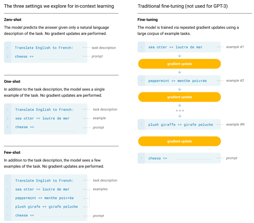
In their research, the authors trained GPT-3, a 175 billion parameter language model, to assess its in-context learning capabilities. They evaluated GPT-3 across diverse NLP tasks and new tasks not included in its training. The model’s performance was tested in three scenarios: few-shot learning (10 to 100 examples), one-shot learning (a single example), and zero-shot learning (only instructions, no examples).

Instruction Tuning (FLAN)
Large-scale language models like GPT-3, developed by Brown and others in 2020, excel at learning from a few examples (few-shot learning). However, they struggle more with learning without any examples (zero-shot learning). For instance, GPT-3 does not perform as well in zero-shot scenarios, especially in tasks like reading comprehension, answering questions, and understanding language inferences, compared to when it has a few examples to learn from. This might be because, without these examples, the models find it difficult to respond to prompts that differ significantly from the data they were trained on.
Google Researches proposed an easy approach to enhance the ability of language models to learn without prior examples (zero-shot learning). They demonstrate that instruction tuning


In their research, the authors found that when using the most effective development template, FLAN in a zero-shot setting outperformed GPT-3 in zero-shot learning on 20 out of 25 datasets. Impressively, it also exceeded GPT-3’s performance in few-shot scenarios on 10 of these datasets. They noted that instruction tuning shows significant effectiveness in tasks that are naturally expressed as instructions, such as natural language inference (NLI), question answering (QA), translation, and converting structures to text. However, it was less effective in tasks inherently structured as language modeling tasks, where instructions might be superfluous. These include commonsense reasoning and coreference resolution tasks typically presented as completing an unfinished sentence or paragraph.
Now, instruction tuning frames all tasks in the form of natural language instruction to natural language response mapping.
Reinforcement Learning from Human Feedback (RLHF)
While instruction tuning is highly effective, it has inherent limitations. For a given input, the target is the single correct answer. This requires formalizing the correct behavior for a given input.

We’re working to teach models more complex behaviors, facing a key challenge: the unchangeable, parameter-less objective function used in fine-tuning. This raises an important question: can we introduce adjustable parameters into this objective function and learn from it?
One of the framework to solve this is RLHF (reinforcement learning human feedback).
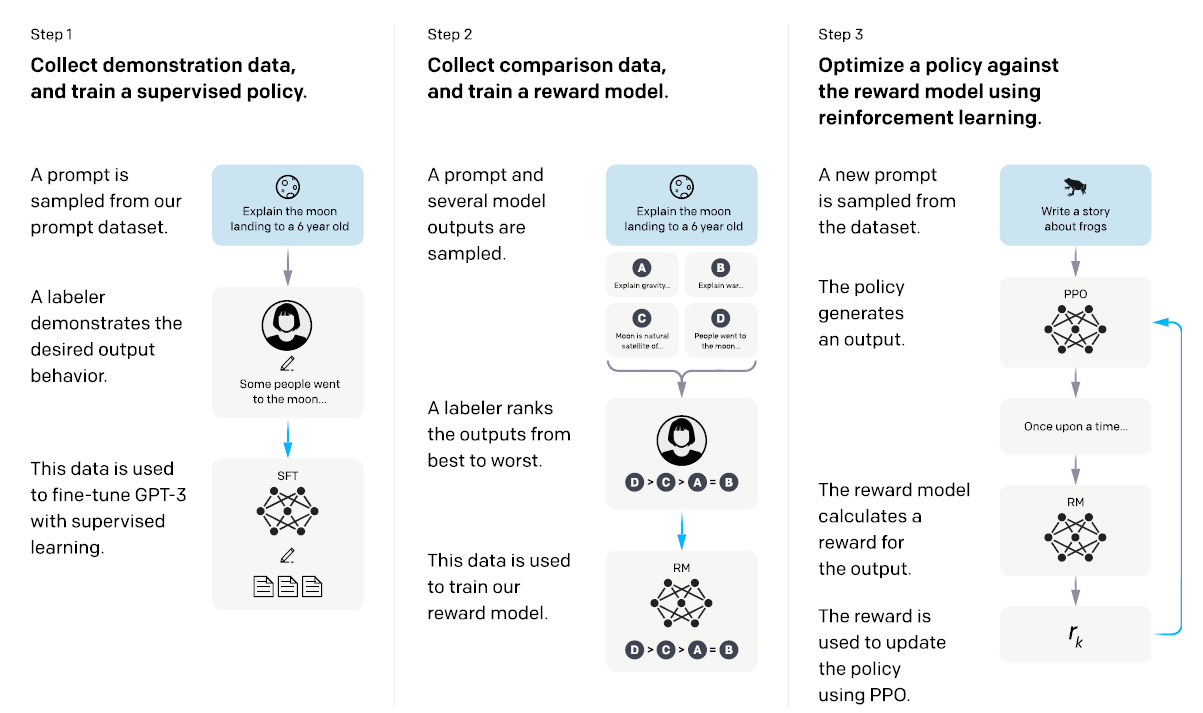
RLHF involves three key steps: collecting human feedback, fitting a reward model, and optimizing the policy with RL. Here, I introduce a straightforward formal framework for Reinforcement Learning from Human Feedback (RLHF), partially based on the framework proposed by Christiano et al. in 2017.
The RLHF process begins with an optional pretraining step, where a base model $\pi_\theta$ with parameters $\theta$ generates a range of examples. In the context of language models, this often involves a language generator pretrained on web text or other datasets.
The first active step involves collecting human feedback. Here, examples are derived from the base model, and feedback is gathered based on these examples. This involves a feedback function mapping each example and random noise to a feedback output, often modeled as
\[x_i \sim \pi_\theta, \quad y_i=f\left(\mathcal{H}, x_i, \epsilon_i\right)\]For instance, in RLHF for chatbots, tasks may consist of conversational pairs with feedback expressed as preferences within these pairs.
The second step is to fit a reward model $\hat{r}_\phi$ using the feedback, aiming to approximate human evaluations as accurately as possible. The training involves minimizing a loss function over a dataset of examples and preferences, often incorporating a regularizer.
Given a dataset of examples and preferences $\mathcal{D}=\left{\left(x_i, y_i\right)_{i=1, \ldots, n}\right}$, the parameters $\phi$ are trained to minimize
\[\mathcal{L}(\mathcal{D}, \phi)=\sum_{i=1}^n \ell\left(\hat{r}_\phi\left(x_i\right), y_i\right)+\lambda_r(\phi)\]$l$ represents an appropriate loss function and $\lambda_r$ acts as a regularizing term.
For instance, when dealing with feedback in the form of pairwise comparisons, suitable loss functions might include the cross-entropy loss or the Bayesian personalized ranking loss.
The final step involves optimizing the policy using reinforcement learning, where the base model is fine-tuned using the reward model $\hat{r}_\phi$.
The new parameters $\theta_{\text {new }}$ are trained to maximize a reward function, which typically includes a regularizer like a divergence-based penalty.
The benefits of RLHF include its ability to allow humans to convey objectives without the need to explicitly define a reward function. This approach helps in reducing reward hacking issues that often arise with hand-specified proxies, making the process of reward shaping more intuitive and implicit. Additionally, RLHF capitalizes on human judgments, which are frequently easier to provide than detailed demonstrations. This has led to its successful application in teaching policies complex solutions in various control environments and in fine-tuning large language models.
However, RLHF does have its own challenges such as reward hacking. More problems can be found in Open Problems and Fundamental Limitations of Reinforcement Learning from Human Feedback.
Training Language Models to follow instructions with Human Feedback (Instruct-GPT)
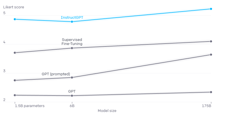
Now, putting everything together, OpenAI Has trained InstructGPT models that surpass GPT-3 in effectively adhering to user intentions and are also enhanced in truthfulness and reduced toxicity.
The effectiveness of InstructGPT in following user instructions was initially assessed by comparing its outputs with those from GPT-3, using labelers for the evaluation. The comparison revealed a clear preference for InstructGPT models, particularly on prompts given to both InstructGPT and GPT-3 models via the API. This preference remained consistent even when modifying the GPT-3 prompts with a prefix to enhance its instruction-following capabilities.
Initially, a dataset of human-authored demonstrations based on prompts from the API is compiled to establish supervised learning baselines. Following this, a larger dataset of human assessments, comparing pairs of model outputs on various API prompts, is gathered. A reward model (RM) is then trained on this dataset to foresee the output preference of the labelers. In the final step, this RM is utilized as a reward function to refine the GPT-3 policy, aiming to maximize this reward by employing the Proximal Policy Optimization (PPO) algorithm.
Discussion
The biggest progress in the past 10 years (or even more) can be summarized in the bitter lesson
- Create weaker inductive biases and scale up
- Do not teach machines how we think we think. Let it learn in a machine’s way

I expect the trend will continue. The path to generalisation was scaling all along but the path to achieving alignment with human values and goals remains a critical and ongoing challenge.
I’m extremely grateful for GPT-4’s existence and the many intelligent, talented individuals who have contributed to its development. This technology is remarkable, possessing a vast range of knowledge in numerous areas, from solving mathematical problems and programming to writing essays and more. I’m hopeful that we can continue to enhance it and eventually develop an Artificial General Intelligence (AGI) that benefits all of humanity.
Thank you so much for reading. If you find this article useful, please consider sharing it with others. : )